TD3 and SAC
TD3 stabilizes DDPG with twin critics, delayed actor updates, and target smoothing; SAC uses maximum-entropy stochastic control.
Abstract. DDPG gave us the basic off-policy actor-critic template for continuous control: replay buffer, critic, deterministic actor , and target networks. The weak point is that the actor directly maximizes an approximate critic, so a critic mistake can pull the policy toward a bad action and make training unstable. TD3 keeps the deterministic DDPG template and stabilizes it with three changes. SAC takes a different route: make the actor stochastic and put entropy directly into the RL objective.
The previous chapter ended with a warning. DDPG is powerful because the actor can follow the critic's action gradient. It is also fragile for the same reason. If the critic mistakenly assigns a high value to a bad action, the actor can move toward it, collect more data near it, and make the error matter even more.
This chapter studies the two standard answers. TD3 asks how to make DDPG more stable while changing as little as possible. SAC asks whether the better answer is not a deterministic actor with external noise, but a stochastic actor trained under a maximum-entropy objective.
Why DDPG Is Unstable
For a replay-buffer transition , DDPG trains the critic with a one-step target:
where is the target critic, and is the target actor. The critic then minimizes the squared Bellman error against this target:
The actor update uses the critic as a maximization objective:
The actor is not comparing several real actions from the replay buffer. It takes the replayed state , proposes its own action , and asks the critic whether that action looks good.
This is useful when is smooth and roughly correct. But the critic is a neural approximation trained by bootstrapping. It can have local errors, sharp peaks, and overestimated regions. DDPG then starts to look like a GAN-style training loop: one network learns a moving objective, and another network learns to exploit that objective.
The most important failure mode is overestimation bias. In DQN, the over noisy action values tends to select actions whose values are accidentally too high. DDPG does not write an explicit , but the deterministic actor plays the same role: it is trained to move toward actions that maximize the learned critic. If the critic overestimates a narrow region, the actor can chase that region.
TD3 is a direct repair of this loop.
TD3: Three Stabilizers for DDPG
Twin Delayed Deep Deterministic Policy Gradient (TD3), introduced by Fujimoto et al. in 2018, keeps the DDPG skeleton:
- a deterministic actor ;
- two action-value critics;
- replay-buffer minibatches;
- target networks with Polyak updates.
The difference is how TD3 builds the bootstrap target and how often it updates the actor.
First: Delay the Actor Update
DDPG updates the critic and actor together. TD3 updates the critic more often than the actor. In the common setting, the critic is updated every gradient step, while the actor and target networks are updated once every critic steps.
The reason is simple. The actor should not chase a critic that is still too noisy. If the critic gets a little more time to fit the current replay data, the actor follows a less erratic value surface.
This gives the "delayed" part of TD3:
The GAN analogy is useful here. If the generator learns too aggressively from a weak discriminator, it can find holes in the discriminator rather than improve the real objective. DDPG has the same shape: the actor can find holes in the critic. Delaying the actor shifts training toward a better critic before the actor moves again.
Second: Smooth the Target Action
DDPG evaluates the target critic exactly at the target actor's next action:
TD3 adds a small clipped noise term to that target action:
Then the critic target is computed at instead of the exact deterministic action. This is called target policy smoothing.
The point is not exploration. The action is not executed in the environment. It is used only inside the Bellman target. Exploration noise affects data collection; target smoothing affects the training label for the critic.
The intuition is local robustness. If an action is good only at one very sharp point, a deterministic actor can exploit that peak. By adding a small perturbation in the target, TD3 asks the critic to value a small neighborhood around the target action. A good action should stay good when changed slightly.
This is also why this noise is not the same as a stochastic policy. A stochastic policy learns a state-dependent distribution: in some states it may be broad, in others nearly deterministic. TD3's target noise is small, fixed by hyperparameters, and not learned. It is a regularizer for the target, not a policy distribution.
Third: Use Two Critics and Take the Minimum
TD3 maintains two critics,
with target copies and . The bootstrap target uses the smaller target value:
Both critics are trained toward this same target form:
The two critics should not be exact copies of each other. Different random initializations already make their approximation errors different. Using differently shuffled minibatches can decorrelate them further, and this is a useful mental model for why the trick works. In the canonical TD3 update, however, both critics are often updated on the same sampled minibatch against the same target form. The algorithm does not require perfect independence; it only needs the two estimates to disagree enough that the minimum can cut off many accidental high spikes.
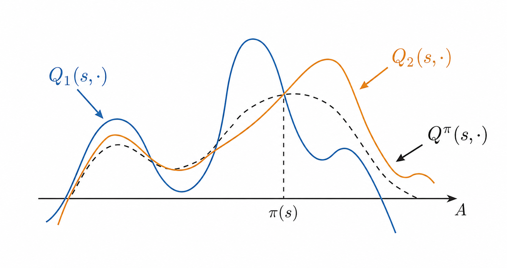
Taking the minimum is deliberately conservative. If one critic has an accidental high spike, the other critic is less likely to have the same spike in the same place. The minimum turns the target into a lower estimate. Underestimation is usually safer than overestimation here because the actor explicitly searches for high critic values. Overestimated actions are chased; underestimated actions are mostly ignored.
The minimum is used when TD3 builds the critic target. The actor update is simpler: it usually maximizes one critic, for example . So the twin trick mainly stabilizes critic learning; it is not a new actor objective.
Putting the three pieces together, the TD3 target is
The actor objective stays close to DDPG:
This is still DDPG, but with safer targets and slower actor movement. It does not solve exploration in a deep way. TD3 still has a deterministic actor, and exploration still comes from external action noise during data collection.
Why Not Just Use a Stochastic Actor?
The natural next question is: why keep adding noise outside a deterministic policy? Why not learn a stochastic policy directly?
Suppose we keep the same critic objective and simply optimize a stochastic policy by
For a fixed state and fixed critic, the best solution is to put all probability mass on the action with the largest . In other words, the optimal policy for this objective is greedy. The stochasticity disappears. So if we want stochasticity to be more than temporary exploration noise, the objective must reward it. SAC does this by adding entropy to the objective itself.
The entropy of a policy in state is
High entropy means the probability mass is spread out. Low entropy means the policy is close to a sharp peak, and in the limit close to deterministic.
In continuous action spaces this is differential entropy, not the finite entropy of a categorical distribution. It can be negative, and it is not bounded by . This is why SAC can use target entropies such as later in the algorithm. The intuition is the same: a very narrow Gaussian has low entropy, while a wider Gaussian has higher entropy.
Maximum-Entropy RL
Soft Actor-Critic optimizes the maximum-entropy objective:
Here is a trajectory generated by policy .
The scalar is the temperature. Large makes entropy more important, so the policy stays broader. Small makes the objective closer to ordinary reward maximization.
This entropy term affects more than the action chosen in the current state. Because entropy is inside the return, a policy can prefer states that leave many good options open later. Imagine a small walking robot at a fork. One path quickly leads to a narrow corridor where only one precise action keeps the robot alive. Another path leads to an open area where several actions still work. If the rewards are similar, standard RL may treat the two paths as almost equal. Maximum-entropy RL gives extra value to the second path because the future policy can stay uncertain there.
The soft greedy policy makes this visible. If two actions have soft values and , their probabilities are proportional to
The better action gets more probability, but the other action does not instantly disappear unless is very small or the value gap is very large.
Using the entropy definition, the same idea can be written along sampled actions as
These two forms say the same thing. If the policy class has an analytic entropy, we can use directly. In a sampled update, one sampled action contributes the Monte Carlo estimate . SAC uses this sampled log-probability in the actor loss and in the critic target.
Not just a larger entropy bonus
In A2C and PPO, entropy is usually an extra regularizer on the policy loss; the critic still estimates the ordinary return. In SAC, entropy is part of the value definition. The Bellman equations themselves change.
There is one conceptual point to be careful about. In a standard MDP, the reward function is part of the environment. It can depend on the state, action, and next state, but it does not depend on the policy we are currently optimizing. The entropy term is different: depends on the whole action distribution chosen by the policy at state . So maximum-entropy RL is not just "the same MDP with a different fixed reward." It changes the objective by adding a policy-dependent term. To handle this cleanly, policy evaluation and policy improvement are rewritten with soft value functions.
Soft Values and Soft Policy Improvement
For a fixed policy , the soft value functions are
The term is the entropy contribution. It is inside the value function, so the critic is no longer learning ordinary return. It learns soft return: reward plus future entropy.
The order is important. is the value before the action is fixed, so it includes the entropy of the policy at state . is the value after we already chose action , so it does not include the current state's entropy term. Instead, receives entropy through the next state's . This is a useful way to read the modified Bellman equations: entropy is like an extra reward attached to having a policy distribution at a state.
Policy improvement changes in the same way. Start with one fixed state and a critic . If we optimized only the expected critic value,
the best policy would put all probability on the action with the largest critic value. That is just the usual greedy policy again. The policy would become deterministic.
Maximum-entropy policy improvement adds the entropy term to this local objective:
The first term still wants high-value actions. The second term prevents all probability mass from collapsing onto one action. We are deriving this because we want to know what "greedy policy improvement" becomes after entropy is added. In ordinary RL, greedy means "put all probability on ." In maximum-entropy RL, greedy becomes soft greedy: better actions get more probability, but nearby or slightly worse actions can still remain possible.
To see the shape of this soft greedy policy, start with the unnormalized score
This score is always positive, and it is larger for actions with larger critic value. But by itself it is not a probability distribution: the scores over all actions do not necessarily integrate to . The normalizer fixes that:
Dividing by turns the scores into a valid density over actions:
This is a softmax-like distribution defined by the critic: actions with higher get higher probability, but lower-value actions can still be sampled (often called a Boltzmann policy in maximum-entropy RL). The max-entropy improvement objective is equivalent to matching the new policy to this distribution:
or, informally,
For the exact optimal soft critic, the same statement is
In continuous control, SAC does not try to represent this exact soft greedy policy directly. Instead, it learns a tractable stochastic actor that approximates it. In practice this actor is usually a squashed Gaussian: the network samples a Gaussian action and then passes it through so the final action stays inside .
The same idea changes Bellman optimality. Its optimality equation uses a hard maximum over next actions:
In maximum-entropy RL, the next-state value is the value of the soft greedy policy. The hard maximum is replaced by a log-sum-exp, or log-integral in continuous action spaces:
This expression is a smooth approximation to . As , it becomes closer to the hard maximum. This is why the values, Bellman equations, and policy improvement step are called "soft."
The SAC Actor and Critic Updates
SAC uses a stochastic actor:
In continuous control, SAC usually uses a squashed Gaussian policy. The policy first samples an unbounded latent action , and then maps it through to get the bounded environment action . The actor is trained with the reparameterization trick:
For a diagonal Gaussian, the two steps are
Here is only an internal sample. The actual action is , which lies in and is the value passed to the critic and the environment. The transformation is differentiable, so the gradient path from back to is still open. When SAC computes , it also accounts for this change of variables.
The actor maximization objective is
Here is maximized. The critic terms below are written as losses because they are minimized.
The actor distribution does not have to be a squashed Gaussian. We could try a richer distribution, for example a mixture of several Gaussians. But the gradient above assumes that the sampled action can be written as a differentiable function of fixed noise. A diagonal Gaussian has exactly this simple form: the network outputs one mean and one standard deviation for each action dimension, samples each dimension independently, and then applies the squashing step. A mixture policy adds a discrete choice of which Gaussian component to use, so the plain pathwise gradient is no longer as clean. Implementations may need a score-function, or REINFORCE-style, term for that part. This is one reason practical SAC usually uses a squashed Gaussian rather than a mixture policy.
The actor wants actions with high soft Q-value, but it also pays a cost for assigning too much probability to one action. This is the part that keeps the policy stochastic during training.
SAC also uses two critics, like TD3. In the modern version, there is no separate network. The soft value is computed implicitly from the critics and the current policy. For a sampled transition , sample a next action
The critic target is
Each critic minimizes
This looks close to TD3, but the meaning is different. TD3 evaluates a deterministic target actor plus small smoothing noise. SAC samples from the stochastic policy and subtracts the log-probability term because entropy is part of the value target.
SAC usually tunes automatically. Instead of hand-picking one temperature for every task, the algorithm sets a target entropy , often near , and updates so that the policy entropy stays near that target. The full dual derivation is not needed here. The practical message is that SAC learns the exploration strength instead of relying only on a hand-tuned noise scale.
SAC Algorithm Shape
The practical SAC loop is:
initialize stochastic actor pi_theta
initialize two critics Q_w1, Q_w2 and target critics
initialize replay buffer D

while training:
    sample action a_t ~ pi_theta(. | s_t)
    execute action and store (s_t, a_t, r_t, s_{t+1}) in D

    sample minibatch from D
    sample next actions a' ~ pi_theta(. | s')
    build soft target with min target Q and - alpha log pi(a' | s')
    update both critics toward the soft target

    update actor to maximize min Q(s, a) - alpha log pi(a | s)
    update alpha toward the target entropy
    Polyak-update target critics
SAC does not need TD3's target policy smoothing. The next action in the target is already sampled from a stochastic policy, and the entropy term discourages collapse to a narrow deterministic peak. SAC also does not rely on external exploration noise in the same way as DDPG and TD3. The behavior policy is the actor itself. SAC also does not use TD3's delayed actor update as a core ingredient. In the standard practical loop, the actor and critics are updated together on replay minibatches; the entropy term makes the actor less likely to collapse into a greedy policy.
TD3 or SAC?
TD3 and SAC share the same off-policy backbone: replay buffer, bootstrapped critics, and target networks. They differ in what they trust.
| Method | Actor | Main stabilizer | Exploration |
|---|---|---|---|
| TD3 | deterministic | conservative twin-Q target, delayed actor update, target smoothing | external action noise |
| SAC | stochastic | maximum-entropy objective, twin soft Q target, learned temperature | inside the policy |
TD3 is the smaller conceptual change from DDPG. It says: keep the deterministic actor, but stop it from exploiting critic errors so easily. The method is often simpler to explain because every piece is a repair of a DDPG failure mode.
SAC changes the objective. It does not want the policy to become deterministic too early. Entropy is not a side bonus; it is part of what the value function means. This gives SAC a cleaner exploration story and usually makes it more robust across random seeds and tasks, at the cost of more machinery: log-probability correction for squashed Gaussians, entropy temperature, and stochastic actor updates.
The papers compared against each other in slightly different historical versions. The TD3 paper compared to an early SAC version; the later SAC follow-up adopted twin Q-functions and automatic temperature tuning. In modern continuous-control practice, SAC is often the stronger default, while TD3 remains the clearest deterministic repair of DDPG.
Full code
The complete runnable example implements SAC on Pendulum-v1, including a squashed Gaussian actor, twin soft critics, automatic temperature tuning, and Polyak target updates:
sac.py
You may also find these implementations useful:
What Comes Next
TD3 and SAC close the off-policy actor-critic line. So far every algorithm we have covered, from Q-learning to SAC, is model-free: it learns a value function or a policy from sampled transitions without ever predicting where the environment will go next. The next chapters take the opposite path. Instead of treating the dynamics as a black box, model-based methods learn (or assume) a model of and use it for planning. That single change reshuffles the design space: replay becomes optional, planning rolls out in imagination, and the exploration question changes shape.