Deep Q-Networks

Abstract. DQN keeps the Q-learning update from the previous chapter but replaces the table with a neural network $Q_\theta(s,a)$. Training naively does not work: the combination of function approximation, bootstrapping, and off-policy data creates instability. DQN solves this with two additions — experience replay and a target network — each addressing a distinct failure mode.

Tabular Q-learning stored one number for every state-action pair. That table is useful for Cliff Walking because the grid has a handful of states and four actions. It breaks down once the state is a continuous observation vector. CartPole has a four-dimensional state; Atari uses raw image frames. In both cases the same exact state may never repeat, so a table cannot generalize.

The DQN move is simple to state: approximate the action-value function with a neural network. Instead of storing $Q(s,a)$ explicitly, learn parameters $\theta$ of $Q_\theta(s,a)$. For a discrete action space, the usual architecture takes a state as input and outputs one scalar per action — a single forward pass yields Q-values for every action simultaneously.

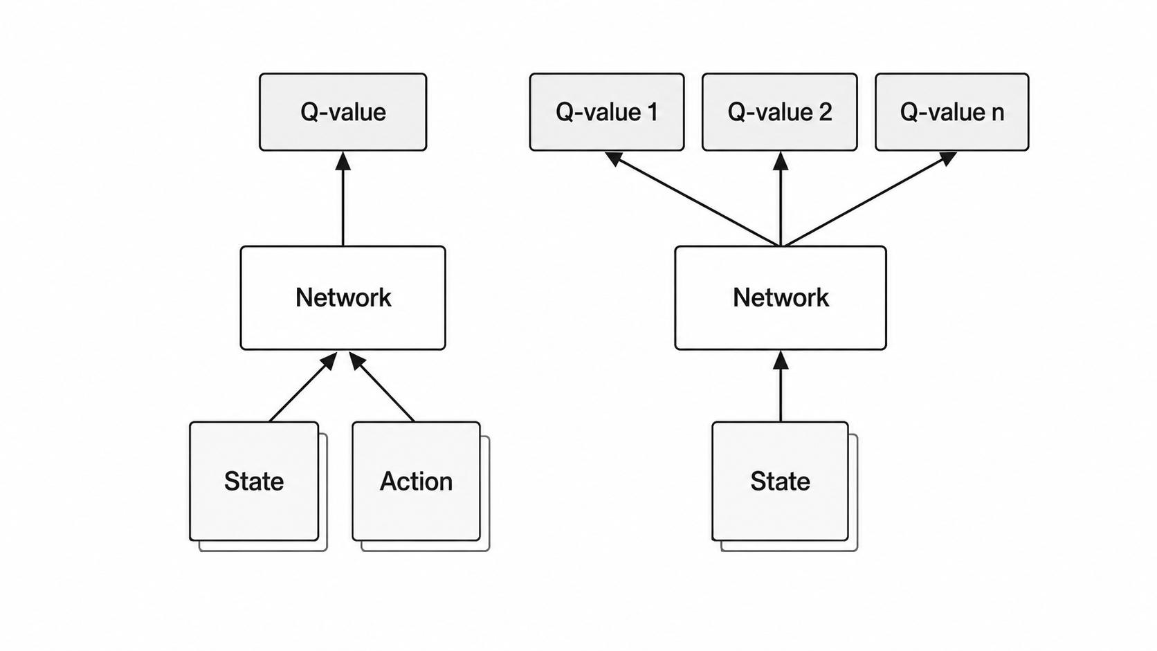
The greedy action is still $\arg\max_a Q_\theta(s,a)$, so DQN remains value-based. The action space must be discrete enough that all action values fit in one forward pass.

Q-Learning as a Regression Problem

From this point we write a transition compactly as $(s, a, r, s')$ — shorthand for $(S_t, A_t, R_{t+1}, S_{t+1})$ with the time index dropped.

The key idea is to cast Q-learning as supervised regression. The Bellman optimality equation (from the MDP chapter) says the optimal action-value function satisfies:

where the expectation is over the random reward $r$ and next state $s'$ from the environment. For a sampled transition $(s,a,r,s')$, the right-hand side gives a single-sample estimate of what $Q_\theta(s,a)$ should be. We use it as a training target and minimize the squared error:

Think of this as supervised learning with a moving label. The input is the state, the output is the Q-value for the chosen action, and $y$ plays the role of a regression target. In ordinary regression the target comes from a fixed dataset; here it is computed from the same network we are trying to train.

One subtlety: gradient must flow only through the prediction $Q_\theta(s,a)$, not through $y$. This is a semi-gradient update: $y$ is treated as a fixed constant for this step, even though it depends on $\theta$. Backpropagating into $y$ would make the update chase a self-referential consistency instead of any external Bellman signal.

The deeper problem is hidden in the target formula: both the prediction $Q_\theta(s,a)$ and the target $y$ depend on the same $\theta$. Every gradient step changes $\theta$, which immediately shifts the target $y$ being chased. The optimizer pursues a moving bullseye: each update shifts the target, so the next update must chase a slightly different value, and the network never settles. In practice this version diverges or oscillates — it simply does not work.

Two structural problems drive the failure. The rest of the chapter addresses each one.

The Deadly Triad

Before naming the fixes, it helps to name the underlying cause. DQN sits on the deadly triad, the danger of instability and divergence arises whenever we combine all of the these three elements:

1. Function approximation — one network represents many state-action values through shared parameters.
2. Bootstrapping — the target contains another learned value estimate, $\max_{a'} Q(s',a')$.
3. Off-policy learning — the data may come from older exploratory policies while the target is greedy.

Each component is individually valuable. Together, especially with nonlinear networks, they can cause oscillation or divergence: updating one part of the network propagates changes to other states through shared weights, those changed estimates become targets for further updates, and stored data may not match the current policy. The deadly triad is not eliminated by DQN, it is tamed by two stabilizers, one for each of the failure modes below.

Problem 1: Correlated Samples

The first problem: transitions collected online are not i.i.d., they are strongly correlated in time. In Atari, consecutive frames differ by only a few pixels: the agent is still in the same room, the same enemies are at nearly the same positions. A minibatch of sequential transitions is essentially the same observation repeated.

This causes two problems. When all samples come from the same part of the game, gradient steps point in roughly the same direction and the network keeps refining the same narrow slice of experience. And when the agent moves to a new region, the weights start fitting the new data and the old knowledge gets overwritten. The network forgets. In practice this shows up as a jagged learning curve: performance rises while the agent stays in one area, then drops when it moves on.

There is a second issue. Each transition is used exactly once and then discarded. This is wasteful: a rare but informative transition that caused a large TD error gets one gradient step and is never seen again.

Experience replay solves both problems. Every transition the agent collects is stored in a finite buffer $\mathcal{D}$:

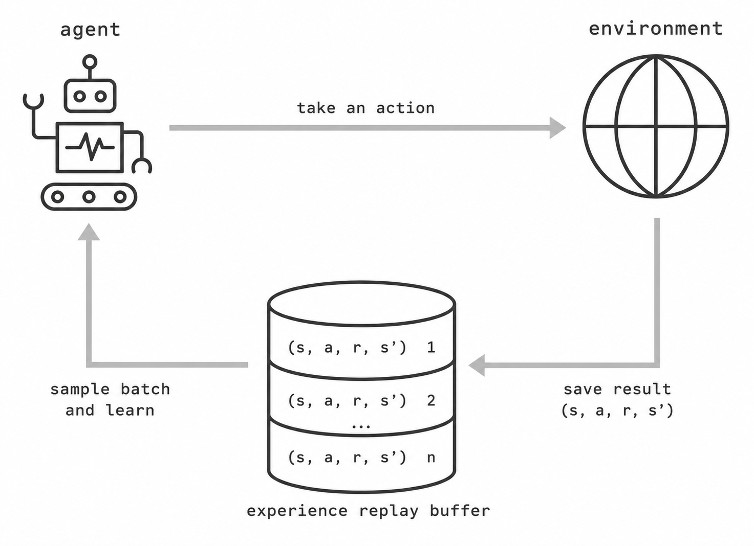
Training draws uniform random minibatches from this buffer. Because transitions are sampled randomly, each minibatch mixes data from different episodes and different stages of training, which breaks the temporal correlations. The same transition can also appear in multiple minibatches, improving data efficiency.

Replay works naturally with Q-learning because Q-learning is off-policy. A transition collected thousands of steps ago, under a larger $\epsilon$ and older weights, is still valid training data: the target is greedy over $s'$ and does not depend on what the old behavior policy would have done next.

Problem 2: The Moving Target

Replay decorrelates the data. It does not fix the other problem: the target $y = r + \gamma \max_{a'} Q_\theta(s', a')$ is computed from the same network that is being updated. Every gradient step moves $\theta$, which moves $y$, which shifts the loss landscape the optimizer was just working on.

Target networks address this by introducing a second, slowly-updated copy of the network. The target network has parameters $\theta^-$ and is used only to compute the bootstrap target. The online network has parameters $\theta$ and is updated at every gradient step. With a frozen $\theta^-$, the target becomes:

Because $\theta^-$ is held fixed for many updates, the target stays still long enough for a block of gradient steps to resemble ordinary fixed-target regression.

The hard copy update overwrites the target network every $C$ gradient steps:

Nature DQN used $C = 10{,}000$. An alternative is the soft Polyak update, applied at every step with a small mixing coefficient $\tau$:

This moves the target network gradually toward the online network. Hard copies are standard for DQN; soft updates appear in the continuous-control methods of Chapter 3 (Actor-Critic).

Exploration with an $\epsilon$ Schedule

DQN collects data with an decaying $\epsilon$-greedy behavior policy. Early in training $\epsilon$ is high so the replay buffer fills with diverse exploratory transitions. Later it decays toward a small floor so the agent mostly exploits the learned Q-function while still collecting some new experience.

The decay rate matters: if $\epsilon$ falls too fast, the buffer fills with near-greedy data before the Q-function is reliable enough to guide it. If it falls too slowly, training is dominated by random actions throughout. In practice a linear decay works well. The right length varies by environment: it should cover at least the period when the Q-function is still too unreliable to guide exploration on its own.

The Training Loop

With replay, a target network, and an $\epsilon$ schedule in place, the full DQN algorithm alternates between acting, storing, and learning:

initialize Q_theta and Q_theta_minus with the same random weights
initialize replay buffer D

for each environment step:
    choose action a with epsilon-greedy(Q_theta(s))
    step environment, observe r, s', done
    store (s, a, r, s', done) in D

    if |D| >= batch_size:
        sample a uniform minibatch from D
        for terminal transitions:     y = r
        for non-terminal transitions: y = r + gamma * max_a' Q_theta_minus(s', a')
        update theta to minimize (y - Q_theta(s, a))^2

    every C steps: copy theta into theta_minus

A few things worth noting. Both networks start with the same weights: the target is not a separate random initialization, just a frozen copy of the online network. Training only starts once the buffer has collected enough transitions; early on the agent simply acts and stores. For terminal transitions the bootstrap term is dropped entirely: the episode is over, so there is no next state to evaluate. The target sync every $C$ steps is the only moment the target network moves; between syncs it is completely frozen.

Example: CartPole

CartPole-v1 is the standard sanity check for deep value-based methods. The state is a four-dimensional vector: cart position, cart velocity, pole angle, and pole angular velocity; and the action space has two choices: push left or push right. The episode ends when the pole falls beyond 12 degrees or the cart drifts off-screen. A perfect episode lasts 500 steps and earns a return of 500.

The Q-network is a two-hidden-layer MLP that maps the four-dimensional state to two Q-values — one per action:

class QNetwork(nn.Module):
    """Two-hidden-layer MLP: state -> Q-value for each discrete action."""

    def __init__(self, state_dim: int, hidden_dim: int, n_actions: int) -> None:
        super().__init__()
        self.fc1 = nn.Linear(state_dim, hidden_dim)
        self.fc2 = nn.Linear(hidden_dim, hidden_dim)
        self.out = nn.Linear(hidden_dim, n_actions)

    def forward(self, x: torch.Tensor) -> torch.Tensor:
        """Forward pass: state -> Q-values over actions."""
        x = F.relu(self.fc1(x))
        x = F.relu(self.fc2(x))
        return self.out(x)

A single forward pass produces Q-values for both actions, and argmax selects the greedy choice. The loss function is the squared TD error from the previous sections, gradient flows only through the online prediction:

def compute_td_loss(
    q_net: QNetwork,
    target_net: QNetwork,
    states: torch.Tensor,
    actions: torch.Tensor,
    rewards: torch.Tensor,
    next_states: torch.Tensor,
    dones: torch.Tensor,
    gamma: float,
) -> torch.Tensor:
    """One-step DQN squared TD-error loss."""
    q_values = q_net(states).gather(1, actions.unsqueeze(1)).squeeze(1)
    with torch.no_grad():
        next_q = target_net(next_states).max(dim=1).values
        targets = rewards + gamma * (1.0 - dones) * next_q
    return F.mse_loss(q_values, targets)

gather picks the Q-value for the action actually taken. torch.no_grad() on the target block ensures $\theta^-$ is treated as a constant: no gradients flow back through the target.

The experiment uses 600 episodes with a hidden dimension of 128, learning rate $2 \times 10^{-3}$, discount $\gamma = 0.99$, and a replay buffer of capacity 10,000. Training starts once the buffer has 500 transitions. The target network syncs every 50 gradient updates. Epsilon decays linearly from 1.0 to 0.05 over the first 5,000 environment steps.

Full code

The complete runnable example, including a replay buffer, target network update, and CartPole DQN training: dqn.py

What Comes Next

DQN made deep value-based RL work by adding replay and target networks to neural Q-learning. The next chapter studies the failure modes that remain: overestimation bias, inefficient uniform replay, and scalar value targets. Each DQN improvement changes one part of the vanilla recipe.