PPO

Abstract. TRPO keeps the policy update inside a hard KL trust region, at the price of a heavy second-order solver. PPO inherits the same local-update idea but replaces the constrained problem with an objective simple enough for plain first-order SGD, while still preventing the policy from moving too far in a single update.

TRPO solved the catastrophic-update problem with a clean recipe: maximize the local surrogate subject to a KL constraint. The price is a heavy update procedure that does not fit standard deep-learning training. Fisher-vector products via conjugate gradient, then a line search, then maybe rejection of the step. On top of that, two practices that are standard in deep RL stop working: you cannot reuse the same rollout batch for several SGD passes (TRPO solves one constrained problem and the batch is done), and the policy and value function cannot easily share a network trunk (TRPO's natural-gradient geometry is defined only on the policy distribution).

Proximal Policy Optimization, introduced by Schulman et al. in 2017, takes the same local surrogate and asks: can we get the same "stay close to $\pi_{\theta_{\text{old}}}$ " effect without solving a constrained problem? The answer comes in two steps. The first step (PPO-Penalty) is to relax the constraint into a regularizer. The second step (PPO-Clip) is to drop the penalty entirely and instead modify the surrogate so the ratio itself stops paying off once it strays too far from $1$ . The clipped variant is the one that became the default, and it is what people usually mean when they say "PPO".

From a Constraint to a Penalty

Recall the TRPO update from the previous chapter. A batch is collected with $\pi_{\theta_{\text{old}}}$ , advantages are estimated with respect to the old policy, and the candidate $\pi_\theta$ is scored by an importance-weighted surrogate. TRPO then maximizes that surrogate subject to a KL constraint:

\max_\theta \; \mathbb{E}_{s,a \sim \pi_{\theta_{\text{old}}}}\!\left[ \frac{\pi_\theta(a \mid s)}{\pi_{\theta_{\text{old}}}(a \mid s)} \, A^{\pi_{\theta_{\text{old}}}}(s,a) \right] \quad \text{s.t.} \quad \bar{D}_{KL}(\pi_{\theta_{\text{old}}} \| \pi_\theta) \le \delta.

A standard way to simplify a constrained problem is to move the constraint into the objective as a regularization. Instead of "maximize the surrogate while keeping the KL below $\delta$ ", we maximize the surrogate minus a KL term:

\mathbb{E}_{s \sim \rho^{\pi_{\theta_{\text{old}}}}}\; \mathbb{E}_{a \sim \pi_{\theta_{\text{old}}}(\cdot \mid s)}\!\left[ \frac{\pi_\theta(a \mid s)}{\pi_{\theta_{\text{old}}}(a \mid s)} \, A^{\pi_{\theta_{\text{old}}}}(s,a) \right] \;-\; \beta\, \bar D_{KL}\!\left(\pi_{\theta_{\text{old}}} \| \pi_\theta\right) \;\longrightarrow\; \max_\theta.

The two expectations are written out separately so the data flow stays explicit. States come from the old policy's visitation $\rho^{\pi_{\theta_{\text{old}}}}$ , actions come from $\pi_{\theta_{\text{old}}}(\cdot \mid s)$ , the advantage $A^{\pi_{\theta_{\text{old}}}}$ is also evaluated under the old policy, and the only piece that moves with the candidate $\theta$ is the new policy $\pi_\theta(a \mid s)$ in the numerator of the ratio. The bar over the KL is a reminder that the divergence is averaged over the same state distribution.

This single-objective form is the PPO-Penalty variant. Compared to TRPO, the practical gain is large. There is no constraint to enforce, no Fisher matrix to approximate, no conjugate gradient, no line search. The whole expression is a differentiable function of $\theta$ , and Adam can optimize it like any other deep-learning loss.

The cost, however, is that this is not the same kind of guarantee TRPO had. TRPO's $\bar D_{KL} \le \delta$ is a hard bound on the policy distribution change. The penalty version only takes an average KL and weighs it against the surrogate. A few states can still see large policy shifts as long as the average stays small, and because $\beta$ is finite, a sufficiently profitable surrogate can always overpower the penalty. In other words, the penalty pulls the new policy back toward the old one, but it does not pin it inside a region the way TRPO did. It is regularization, not a trust region. The penalty form does the job sometimes but is usually outperformed by the next idea, which attacks the ratio directly.

PPO-Clip

The clipped variant takes a different angle on the same problem. Instead of regularizing through a separate KL term, it modifies the surrogate so that the ratio itself stops paying off once it leaves a small neighborhood of $1$ .

The importance ratio is the same object as in TRPO. For a sampled $(s_t, a_t)$ pair, define

r_t(\theta) := \frac{\pi_\theta(a_t \mid s_t)}{\pi_{\theta_{\text{old}}}(a_t \mid s_t)}.

If $r_t(\theta) = 1$ , the new policy assigns the same probability to the action as the old one. If $r_t(\theta) > 1$ , the sampled action became more likely under the new policy; if $r_t(\theta) < 1$ , it became less likely. Multiplying by the advantage gives the surrogate $r_t(\theta)\, A^{\pi_{\theta_{\text{old}}}}(s_t,a_t)$ , which is exactly the importance-weighted term from TRPO.

There are two ideas to be discussed. Firstly, clipping the importance ratio. Define the clipped ratio

r_t^{\text{clip}}(\theta) := \operatorname{clip}\!\bigl(r_t(\theta),\, 1-\epsilon,\, 1+\epsilon\bigr),

and the corresponding naive surrogate

L^{\text{clip}}(\theta) := \mathbb{E}_{t}\!\left[r_t^{\text{clip}}(\theta)\, A^{\pi_{\theta_{\text{old}}}}(s_t,a_t)\right].

The clip function leaves $r_t(\theta)$ untouched while it stays inside $[1-\epsilon,\,1+\epsilon]$ , and returns the boundary value $1\pm\epsilon$ as soon as the ratio tries to leave that interval. The typical choice is $\epsilon = 0.2$ , which means the new policy is allowed to make the sampled action up to about $20\%$ more or less likely than before. Past the boundary the surrogate stops changing with $\theta$ , so the gradient in that direction goes to zero.

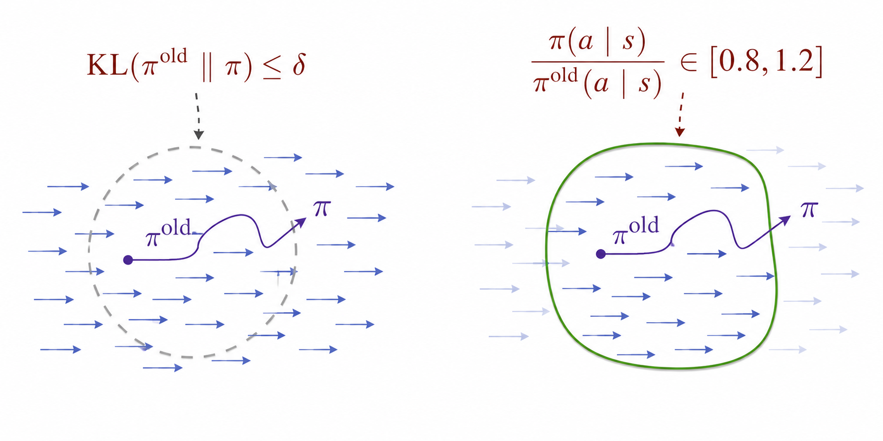
Comparison of default and clipped surrogate function .

Visually, you can see is as a region among $\pi_{\theta_{\text{old}}}$ . In the default surrogate function the gradient can move the $\pi_{\theta}$ far from the $\pi_{\theta_{\text{old}}}$ and clipping helps to avoid it: whenever the policy is out of the region $[1-\epsilon, 1+\epsilon]$ , for example $[0.8, 1.2]$ , the objective stops rewarding movement, which produces a similar effective neighborhood much easier.

So, clipping is already prevents the ratio from running away, but it has a problem: the cap is symmetric. It limits the reward for helpful over-moves, but it equally hides the cost of harmful ones. If a minibatch pushes the policy in a direction that actually hurts the surrogate, we still want the loss to push back; with plain clipping, that pushback disappears as soon as $r_t$ leaves the interval.

The fix is the second operation: take the pessimistic minimum of the unclipped and clipped surrogates,

L^{\text{PPO}}(\theta) := \mathbb{E}_{t}\!\left[ \min\!\left( r_t(\theta)\, A^{\pi_{\theta_{\text{old}}}}(s_t,a_t),\; r_t^{\text{clip}}(\theta)\, A^{\pi_{\theta_{\text{old}}}}(s_t,a_t) \right) \right].

The min always picks the more pessimistic of the two terms. The behavior splits into four cases by the sign of the advantage and the side of the safe interval the ratio drifted to; for example let's stick to $[0.8, 1.2]$ clipping:

Advantage sign	Update direction	Where the ratio ended up	Gradient
$A^{\pi_{\theta_{\text{old}}}}(s_t,a_t) \ge 0$	$\pi_\theta(a_t \mid s_t)\;\uparrow$	$r_t(\theta) > 1.2$	$0$
$A^{\pi_{\theta_{\text{old}}}}(s_t,a_t) \ge 0$	$\pi_\theta(a_t \mid s_t)\;\uparrow$	$r_t(\theta) < 0.8$	same as unclipped
$A^{\pi_{\theta_{\text{old}}}}(s_t,a_t) < 0$	$\pi_\theta(a_t \mid s_t)\;\downarrow$	$r_t(\theta) > 1.2$	same as unclipped
$A^{\pi_{\theta_{\text{old}}}}(s_t,a_t) < 0$	$\pi_\theta(a_t \mid s_t)\;\downarrow$	$r_t(\theta) < 0.8$	$0$

The gradient vanishes only in the two rows where the policy has already over-shot in the direction the advantage wanted. In the other two, the ratio drifted against the advantage, and the unclipped gradient stays at full force. That asymmetry is the whole trick of the min: clipping switches off the gradient only when there is nothing more to gain, and never when the loss should still be pushing back.

PPO does not simply clip every ratio and multiply by the advantage. The min matters. If a proposed change hurts the surrogate, PPO lets the loss feel that full damage. It only caps the artificial gain from pushing a helpful direction too far.

To conclude, adding all together gives us following objective:

\mathbb{E}_{t}\!\left[ \min\!\left( r_t(\theta)\, A^{\pi_{\theta_{\text{old}}}}(s_t,a_t),\; r_t^{\text{clip}}(\theta)\, A^{\pi_{\theta_{\text{old}}}}(s_t,a_t) \right) \right] \;-\; \beta\, \bar D_{KL}\!\left(\pi_{\theta_{\text{old}}} \| \pi_\theta\right) \;\longrightarrow\; \max_\theta.

In practice, clipping often does all the work on its own: a grid search over $\beta$ can land on $\beta = 0$ , which makes the KL term redundant. Some implementations drop the KL penalty entirely for simplicity, but we keep it in our code.

Actor-Critic Implementation

PPO is often introduced as a policy-gradient algorithm, but practical PPO is an on-policy actor-critic method. The actor is the policy network $\pi_\theta(a \mid s)$ with parameters $\theta$ . The critic is a separate network $V_\phi(s)$ with its own parameters $\phi$ , predicting the discounted return from state $s$ (or it can share a trunk with the policy and live as a second head, either way it is a function of $s$ alone, not of $(s, a)$ ).

These two networks correspond to two independent training jobs on the same rollout batch, which is collected by running $\pi_{\theta_{\text{old}}}$ in the environment for a fixed number of steps and storing each transition $(s, a, r)$ :

The policy is updated by maximizing $L^{\text{PPO}}(\theta)$ from the previous section.
The critic is updated by minimizing the mean-squared regression loss between its prediction $V_\phi(s_t)$ and a per-step target $\hat Q(s_t, a_t)$ :

L_{\text{value}}(\phi) = \mathbb{E}_t\!\left[\bigl(\hat Q(s_t, a_t) - V_\phi(s_t)\bigr)^2\right].

This is the same shape as the DQN regression loss from the value-based chapter, only with learnable $V_\phi$ instead of $Q_\theta$ on the prediction side. $\mathbb{E}_t$ is the average over timesteps in the rollout batch. $\hat Q(s_t, a_t)$ here is the per-step empirical estimate of the old policy's action-value $Q^{\pi_{\theta_{\text{old}}}}(s_t, a_t)$ , computed once per timestep in the rollout batch. The remaining design choice is how to build $\hat Q$ .

Three natural candidates for $\hat Q$ , each a different bias-variance trade-off:

Monte Carlo return $\hat Q(s_t, a_t) = G_t = \sum_{k=0}^{T-t} \gamma^k r_{t+k}$ . Unbiased, exactly what the critic is trying to predict on average. But every future reward contributes noise to the target at time $t$ , so the variance is large over long horizons.
TD(0) target $\hat Q(s_t, a_t) = r_t + \gamma V_{\phi_{\text{old}}}(s_{t+1})$ . Low variance, because it only looks one step into the future, but biased: the bootstrap $V_{\phi_{\text{old}}}$ on the right is itself wrong by some amount, and that error propagates into the target.
GAE-based $\lambda$ -return $\hat Q(s_t, a_t) = V_{\phi_{\text{old}}}(s_t) + \hat A_t^{\text{GAE}(\gamma,\lambda)}$ . A $\lambda$ -blend of the previous two: at $\lambda = 1$ it reduces to the Monte Carlo return, at $\lambda = 0$ to TD(0), and at the typical $\lambda \approx 0.95$ it sits in the sweet spot — most of the multi-step credit assignment of MC, most of the variance damping of TD.

PPO defaults to the third. The advantage estimate $\hat A_t^{\text{GAE}(\gamma,\lambda)}$ already shows up in the policy loss, and was introduced in the TRPO chapter as

\hat{A}_t^{\text{GAE}(\gamma,\lambda)} = \sum_{l=0}^{T-t-1}(\gamma\lambda)^l\,\delta_{t+l}^V, \qquad \delta_t^V = r_t + \gamma V_{\phi_{\text{old}}}(s_{t+1}) - V_{\phi_{\text{old}}}(s_t).

So building $\hat Q$ on top of it costs nothing extra: by the same $Q = V + A$ identity, we can use $\hat Q(s_t, a_t) = V_{\phi_{\text{old}}}(s_t) + \hat A_t^{\text{GAE}}$ . The critic then regresses the live $V_\phi(s_t)$ onto these fixed returns.

The on-policy setting also helps here. Unlike Q-learning, where TD targets have to bootstrap through values of states visited under whatever stale behavior policy lives in the replay buffer, PPO's rollouts are coherent and recent, so multi-step returns are reliable.

In the original paper you can see a final compound objective, which is (approximately) maximized each iteration:

L^{\text{PPO+value+S}}_t(\theta, \phi) = \hat{\mathbb{E}}_t\!\left[ L^{\text{PPO}}_t(\theta) - c_1\, L_{\text{value}}(\phi) + c_2\, H\!\bigl(\pi_\theta(\cdot \mid s_t)\bigr) \right].

The three pieces:

$L^{\text{PPO}}_t(\theta)$ — the per-step clipped policy surrogate from the PPO-Clip section. Maximized.
$L_{\text{value}, t}(\phi) = \bigl(\hat Q(s_t, a_t) - V_\phi(s_t)\bigr)^2$ — the per-step critic regression loss we just derived. Subtracted with weight $c_1$ , so it is minimized in the same step.
$H\!\bigl(\pi_\theta(\cdot \mid s_t)\bigr)$ — the entropy of the policy at $s_t$ . Added with weight $c_2$ to reward spread-out action distributions, which slows collapse of the policy to a near-deterministic strategy. So this term just makes the policy to be more stochastic and closer to uniform distribution over actions. The bonus is inherited from A3C (Mnih et al., 2016) and is optional: the original PPO paper uses it on Atari with $c_2 = 0.01$ but disables it on MuJoCo continuous control. We follow the same default and leave it off.

Training Loop

A PPO iteration has a simple shape:

initialize policy pi_theta and value function V_phi

while not converged:
    pi_old    <- pi_theta                          # snapshot policy for this iteration
    V_phi_old <- V_phi                             # snapshot value network for this iteration
    Batch rollout <- generate(pi_old)                          # collect rollout (s, a, r) under pi_old

    compute V_phi_old(s) for all s in D            # cached snapshot values, no gradient
    compute advantages A_hat for all (s, a) in D   # via GAE, using V_phi_old
    compute value targets Q_hat                    # Q_hat = V_phi_old + A_hat
    normalize advantages within D

    for epoch in 1..n_ppo_epochs:
        for batch in batches(D):
            for each (s, a) in batch:
                compute importance ratio r_t(theta, s, a)
                compute clipped ratio r_t_clip(theta, s, a)
            compute clipped policy loss            # using r_t, r_t_clip, A_hat
            compute value regression loss          # against Q_hat
            (optional) compute entropy bonus
            combine into one scalar loss; backprop; optimizer step

    discard D

The hyperparameters PPO uses are ordinary: $\epsilon \approx 0.2$ for the clip range, $\gamma = 0.99$ for the discount, $\lambda = 0.95$ for GAE, 4–10 SGD epochs per rollout batch, minibatches of a few dozen to a few hundred samples, Adam with a learning rate around $3 \times 10^{-4}$ , and entropy coefficient $c_2 \approx 0.01$ if the bonus is enabled. Our PPOConfig in ppo.py uses exactly these defaults, with the entropy bonus turned off.

The non-obvious bit is hidden in the inner loop: each rollout batch is passed through several full epochs of minibatch SGD. With an unclipped surrogate this would be dangerous, because every step pushes the policy further from $\pi_{\theta_{\text{old}}}$ , and after a couple of passes the batch no longer represents the distribution the current policy induces. Importance ratios blow up, variance explodes, and the update turns destructive. This is the "destructively large policy updates" failure mode the PPO paper points to as the motivation for trust-region methods. Clipping defuses it automatically: as soon as a sample's ratio leaves $[1 - \epsilon, 1 + \epsilon]$ in the direction the advantage wants to push, the objective flatlines on that sample. Early SGD steps move the policy in directions the data still supports; later steps see ratios already at the boundary and stop pulling further. The batch is self-limiting, which means that by the time the policy has drifted enough for the importance weights to be unreliable, the loss in those directions has already turned off. That is what makes K epochs over a single batch a stable operation. Note that this does not make PPO off-policy: the batch is fresh data from $\pi_{\theta_{\text{old}}}$ , not replay from many old policies.

Stepping back, PPO is not the most sample-efficient method in every setting: off-policy actor-critic algorithms can squeeze more out of replay data, and specialized methods can beat it on particular benchmarks. What made it the default is the combination of stability, implementation simplicity, and compatibility with standard deep-learning tooling. PPO became the default optimizer in early RLHF pipelines for language models also because of its operational shape: a fresh on-policy batch, advantage estimates, several stable minibatch updates, and a built-in cap on how far the policy can drift. There the policy is the language model itself, and a KL penalty to a reference model takes over the role of the trust region. The takeaway is not that PPO is magically optimal: it is that a small objective-level constraint on the probability ratio is enough to make ordinary SGD work for on-policy policy optimization.

Full code

The complete runnable example, including CartPole rollouts, GAE, old log-prob storage, minibatch updates, and the PPO-Clip loss: ppo.py

What Comes Next

PPO closes the on-policy policy-based line for now: collect fresh rollouts, estimate advantages, take several clipped SGD epochs, then discard the batch. The next chapters ask a different question: can we build actor-critic methods but as off-policy algorithms? DDPG, TD3, and SAC introduced in the next chapters answer this question.